What is Sepeculative Decoding

Ref：Fast Inference from Transformers via Speculative Decoding

Speculative Decoding

Overview

We have a slow, big target model $M_p$, inference from which we're trying to accelerate (distribution $p(x)$). We also have a quick, efficient approximation model $M_q$ (distribution $q(x)$). Core idea:

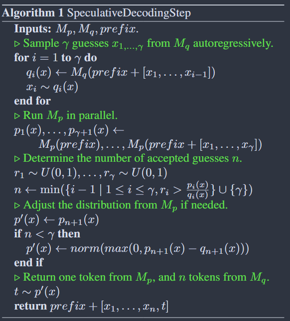
1. We use the efficient model $M_q$ to generate $\gamma$ completions.
2. We use the target model $M_p$ to evaluate all these guesses $in\space parallel$, accepting all those that can lead to an identical distribution.
3. If one token is rejected, we make adjustments to the distribution and then sampling an additional token.

Speculative Sampling

For each sample token:

• If $q(x)\leq p(x)$, we accept this sample
• Or, we reject it with probability $1-\frac{p(x)}{q(x)}$.
  • If it's rejected, we also reject all tokens after this one and make an adjustment to the distribution and sample one correct token.

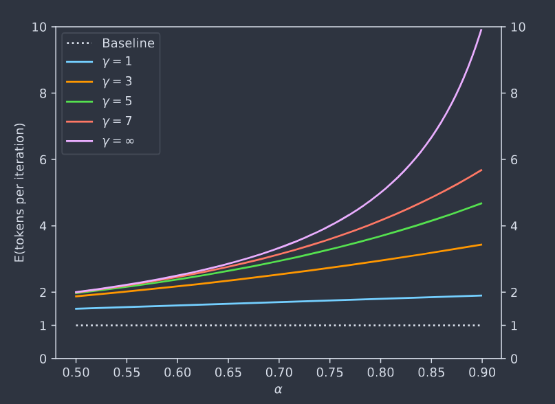
In the best-case scenario, we can generate $\gamma+1$ tokens in a parallel run of the target model $M_p$ (the worst is $1$ token, but we know the traditional method also get only $1$ token).

Pseudo-code:

Here are something notable:

• $p_1(x),...,p_{\gamma + 1}\leftarrow M_p(prefix),...,M_p(prefix+[x_1,...,x_\gamma])$

  This operation is being done in parallel. We concat $prefix$ with the $\gamma$ guess tokens to make a complete array and input to the target model $M_p$ all at once.

  Causal Mask mechanism of the Transformer allows model to output the probability distribution of these $\gamma+1$ positions in parallel during one signal forward pass computation.

• $r_1\sim U(0,1),...,r_\gamma \sim U(0,1)$

  $n\leftarrow \text{min}(\{i-1\mid1\leq i\leq \gamma,r_i\gt\frac{p_i(x)}{q_i(x)}\}\cup\{\gamma\})$

  Generate $\gamma$ uniformly distributed random numbers between $0$and $1$, then we check these numbers to see if token $x_i$ need to be rejected.

  If $p_i(x_i)\geq q_i(x_i)$, we can see $\frac{p_i(x)}{q_i(x)}$ will be greater than $1$, so it won't be rejected.

  $n$ is the index immediately preceding the first rejected position (also it's the number of consecutively accepted tokens).

• $p'(x)\leftarrow \text{norm}(\text{max}(0,p_{n+1}(x)-q_{n+1}(x)))$

  If $n\lt\gamma$, meaning the $(n+1)$the guess was rejected. To correct this error, we do the above operation to generate a new distribution $p'(x)$.

Prove that $x$ sampled in this way indeed $x\sim p(x)$

See Appendix

Analysis

Number of Generated Tokens

To analyze the expected number of tokens produced by a single run of Algorithm 1, we first have the following definition:

• The $acceptance\space rate \space \beta_{x\lt t}$, given a prefix $x_{\lt t}$, is the probability of accepting $x_t\sim q(x_t\mid x_{\lt t})$ by speculative sampling.
• $\alpha = E(\beta)$ is to show how well $M_q$ approximates $M_p$

The result is actually a geometric variable. Let's say that we accept $k$ tokens, the probability of this case:

[!tip]

We get see $E(\#generated\ tokens)$ as the sum of contribution of each position:

• For the first token, the contribution is 1 because $M_p$ always generates at least once token.
• For the second token, the contribution is $\alpha$, meaning the first one is accepted.
• For the $(\gamma+1)$th token, the contribution is $\alpha^\gamma$
• So: $E(\#generated\ tokens)=1+\alpha+\alpha^2+...+\alpha^\gamma=\frac{1-\alpha^{\gamma+1}}{1-\alpha}$

Calculating $\alpha$

• Definition: $D_{LK}(p,q)=\sum_x\mid p(x)-M(x)\mid=\sum_x\mid q(x)-M(x)\mid$ where $M(x)=\frac{p(x)+q(x)}{2}$

• Lemma: $D_{LK}(p,q)=1-\sum_x\text{min}(p(x),q(x))$

  $Proof$. $D_{LK}(p,q)=\sum_x\mid p(x)-M(x)\mid=\sum_x\frac{\mid p-q\mid}{2}=1-\sum_x\frac{p+q-\mid p-q\mid}{2}=1-\sum_x\text{min}(p(x),q(x))$

[!tip]

In case you forget, $\sum p=\sum q = 1$, so we have $\sum\frac{p+q}{2}=\sum\frac{p}{2}+\sum\frac{q}{2}=1$

• Corollary:

  • $D_{LK}(p,q)=0\iff p=q$
  • $D_{LK}(p,q)=1\iff p\ and\ q\ have\ disjoint\ support$

• Theorem: $\beta=1-D_{LK}(p,q)$

  $Proof.$ $\beta=E_{x\sim q(x)}\begin{cases}1&q(x)\le p(x)\\\frac{p(x)}{q(x)}&q(x)\gt p(x)\end{cases}=E_{x\sim q(x)}\text{min}(1,\frac{p(x)}{q(x)})=\sum_x \text{min}(p(x),q(x))$

• Corollary: $\alpha=1-E(D_{LK}(p,q))=E(\text{min}(p,q))$

Walltime Improvement

• Definition: $c$ is the ratio between the time for a single run of $M_q$ and the time for a single run of $M_p$

• The expected improvement factor in total walltime is $\frac{1-\alpha^{\gamma+1}}{(1-\alpha)(\gamma c+1)}$

  $Proof.$

  Let's say $T$ is the cost of running a single step of $M_p$. For each run of Algorithm $1$ costs $Tc\gamma+T$ (running $M_q$ $\gamma$ times and running $M_p$ once). On average we produce $\frac{1-\alpha^{\gamma+1}}{1-\alpha}$ tokens. So the overall expected cost for producing a token with Algorithm $1$ is $tmp=(Tc\gamma+T)/\frac{1-\alpha^{\gamma+1}}{1-\alpha}=\frac{(c\gamma+1)(1-\alpha)}{1-\alpha^{\gamma+1}}T$. So the factor is $T/tmp=\frac{1-\alpha^{\gamma+1}}{(1-\alpha)(\gamma c+1)}$

Number of Arithmetic Operations

Similar to walltime improvement so I just pass this one.

Choosing $\gamma$

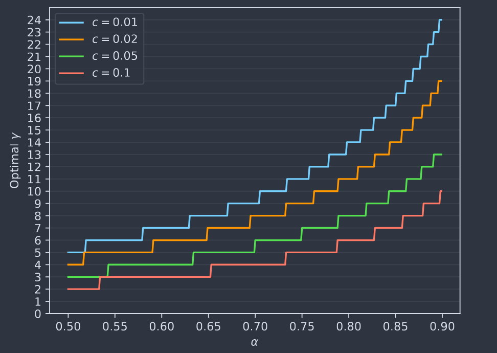
The optimal $\gamma$ should be the one maximizing the walltime improvement equation (enough compute resources).

[!NOTE]

This $\gamma$ can be modified dynamically according to the value of $\beta$

Appendix

To understand this proof, you need first read the Corollary in Calculate $\alpha$ about $\beta$.

First we have $p'(x)=norm(max(0,p(x)-q(x)))=\frac{p(x)-min(q(x),p(x))}{\sum_{x'}(p(x')-min(q(x'),p(x')))}=\frac{p(x)-min(q(x),p(x))}{1-\beta}$

Now:

Where:

And:

Overall: